Modelling Standardisation Series - 1 - Declustering

Declustering techniques help understand the sampling bias that usually tends to target better grades.

Such analysis will give a better insight into the impact of the sampling irregularity on the resulting appreciation of the grade distributions.

The following article shows how declustering can be implemented into a standardised workflow.

The theory behind declustering functions

The fact that the sampling is never perfectly regular, means the naive sample distribution will always be biased to a certain extent. The declustering tools help understand this bias and better forecast a block model distribution.

The declustering consists of assigning to each point a weight value and computing the weighted statistics.

Low weights are assigned to the points that formed spatial clusters while high weights are given to isolated points. Common practice with declustering is to test several window sizes and retain the one giving the minimum declustered average (paper from Pyrcz and Deutch)

The most common techniques for declustering are “Moving Window”, “Grid Cell”, and “Polygon Declustering”.

The python library GeoLime offers access to the most commonly used “Moving Window” and “Grid Cell” algorithms.

GeoLime implementation of declustering functions

While there seem to be several populations in the Ni distribution, we intentionally leave the data un-domained for the sake of simplicity.

The data is composited at 2m.

The following python code is implemented using GeoLime library functions to compute the declustered statistics.

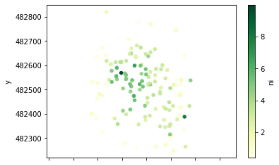
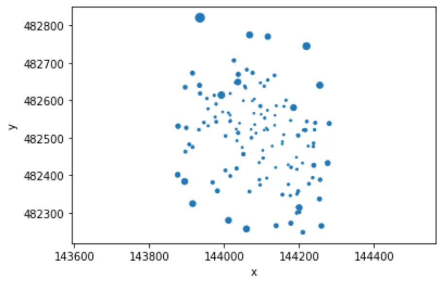
# we can plot the spatial distribution of the data
drillholes.collar.plot.scatter('x','y', c='ni', cmap='YlGn')
plt.axis('equal')

(143855.53525330112, 144300.48674669888, 482218.78769692953, 482848.9034906873)

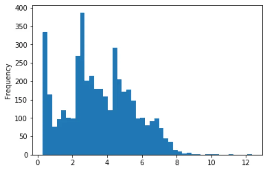
# and have a look at the nickel distribution
f = drillholes.df['ni'].plot.hist(bins=45)

# we test different cell sizes to look for the minimum declustered mean
ni_means, cell_sizes, fig = test_cell_sizes_for_declus(
    drillholes,
    method='cell_declustering'
    )
plt.show()

# Let's keep the cell size for which the declustered mean is the smallest
ind = np.where(ni_means == np.nanmin(ni_means))
cell_size = cell_sizes[ind][0]\

print(f'-------> minimum declustered nickel mean of {ni_means[ind][0]}% is obtained for a grid cell size of {cell_size}m')

-------> minimum declustered nickel mean of 2.6872273714515114% is obtained for a grid cell size of 200.0m

​

Based on an automatically found drilling pattern, we run a declustering algorithm to get the sample declustered weights

drillholes.df['declus_weight'] = plm.cell_declustering(drillholes,
                                                        size_x=cell_size,
                                                        size_y=cell_size,
                                                        size_z=2,
                                                        var='ni',
                                                        nb_off=10)

# Map of drillhole's weights
collars = drillholes.df.groupby(['holeid', 'x', 'y'], as_index=False).mean()
collars.plot.scatter('x','y', s=collars.declus_weight\*10)
plt.axis('equal')

(143855.5354109347, 144300.48573979194, 482218.7895127667, 482848.9122110448)

# Plot the histogram with no weight vs with declustering weights
f = weighted_hist(drillholes.df, 'ni', drillholes.df['declus_weight'])

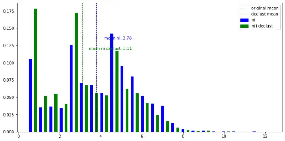
The overall mean is brought down from 3.79% to 3.11%.

The naive mean in nickel was overestimated as it is often the case when considering that targeted drilling will most likely be more present in mineralised zones.

Analysis of results

The declustered distribution shows that a ‘raw’ approach to the drillhole statistics would lead to a miss-interpretation of the deposit’s economics.

It is quite usual to have, at a global scale (without domains), an over-representation of the high-grade zones and an under-representation of the low-grade zones, as the drilling tends to confirm the mineralisation. In that case, we can assume the naive distribution will show an overestimation of the mean of the deposit.

However, it is to note that at a smaller scale, after the definition of the domains, grade should be more stationary and the irregularity of the sampling might be over or underestimating the grade.

It is also worth mentioning that this quick analysis does not take into account the support effect, which will be discussed in a further article.

Most importantly, the declustering results are very sensitive to the size and orientation of the window considered. The results are indicative of a trend, but should not be regarded as a good estimator of a final grade distribution.

A spatial interpolator, such as ordinary kriging will provide a much more reliable analysis.

UX and automation of processes

The workflow has been ported to DeepLime’s GeoPortal.

Authorised users can run the declustering function without having to worry about code or parameters that can be automatically inferred (such as the declustering window size).

While it can be argued that one will lose in flexibility of options, this implementation is customised to suit a particular geological environment, with the aim of standardising the declustering analysis for any new data being looked at.